Table of Contents

1. CT Head Interpretation
2. Intracranial Hemorrhage Detection by 3D Voxel Segmentation on Brain CT Images
3. Deep Learning for Hemorrhagic Lesion Detection and Segmentation on Brain CT Images
4. Autoencoders for unsupervised anomaly segmentation in brain MR images: A comparative study
5. Medical Image Segmentation: A Review
6. Intensity population based unsupervised hemorrhage segmentation from brain CT images - 2018
7. Multi-view fusion segmentation for brain glioma on CT images - 2021
8. Accelerating Prediction of Malignant Cerebral Edema After Ischemic Stroke with Automated Image Analysis and Explainable Neural Networks - 2021
9. Automated medical image segmentation techniques
10. Application of Machine Learning to Automated Analysis of Cerebral Edema in Large Cohorts of Ischemic Stroke Patients
11. Quantitative Serial CT Imaging-Derived Features Improve Prediction of Malignant Cerebral Edema after Ischemic Stroke
12. Enhanced Detection of Edema in Malignant Anterior Circulation Stroke (EDEMA) Score A Risk Prediction Tool

1. CT Head Interpretation

Computed tomography (CT) scanning involves the use of X-rays to take cross-sectional images of the body.

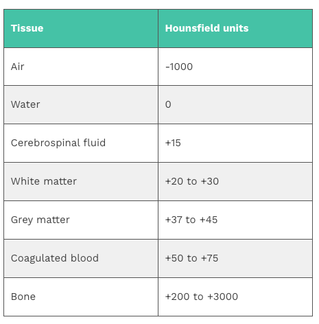
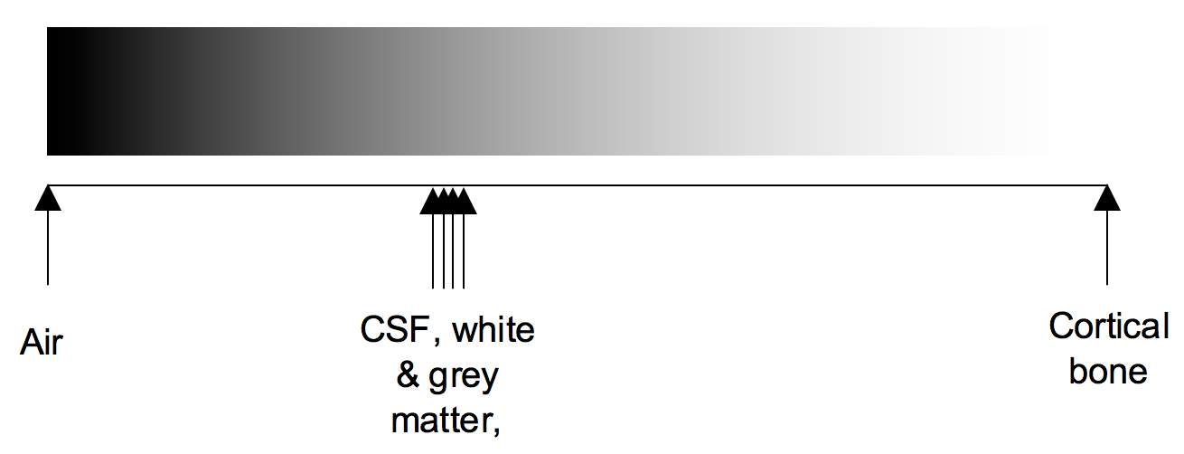
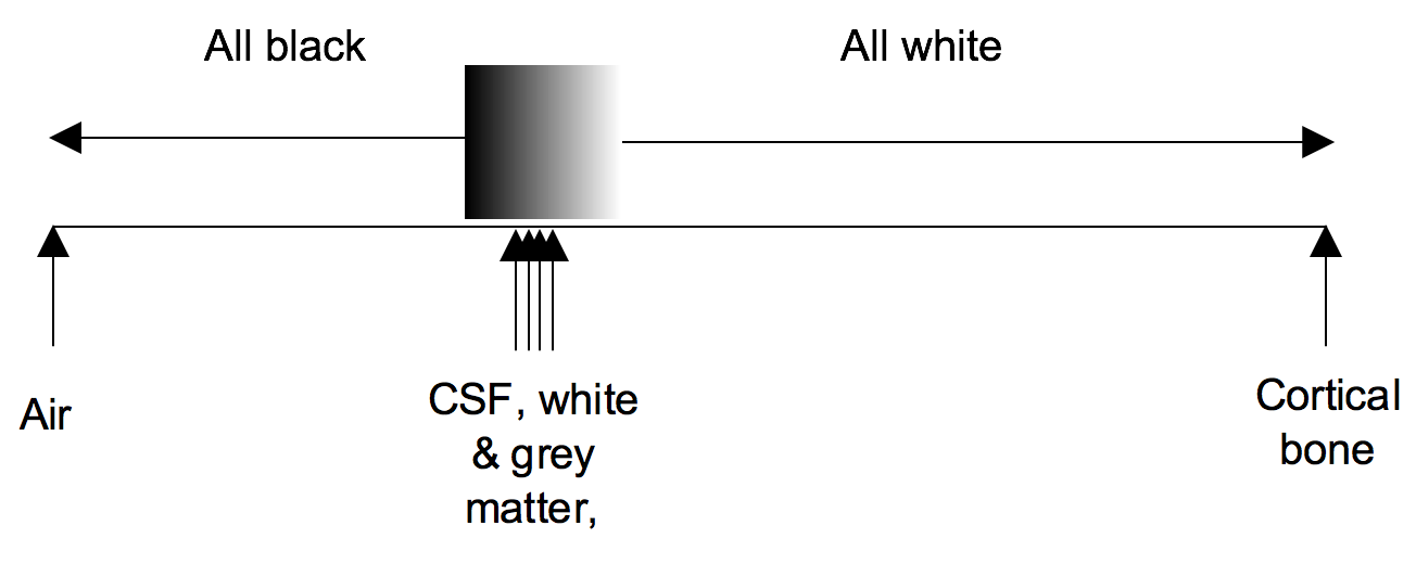
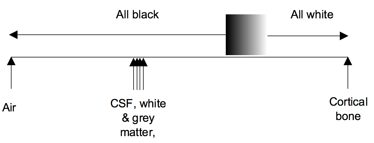
The extent to which a material can be penetrated by an X-ray beam is described in terms of an attenuation coefficient which assesses how much a beam is weakened by passing through a voxel of tissue (voxel = volumetric pixel). These values are frequently expressed as Hounsfield units (HU).

Windowing

Windowing (also known as grey-level mapping) is the process of changing the location and width of the available greyscale in order to optimise discrimination between tissues.

Blood

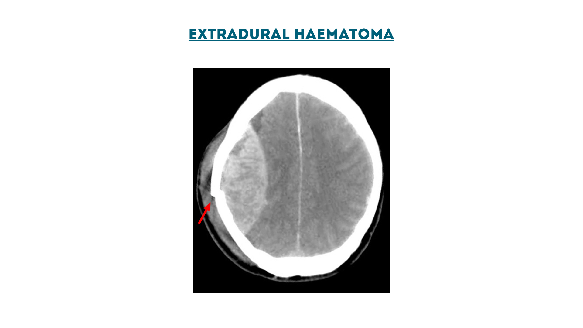
Extradural haematoma

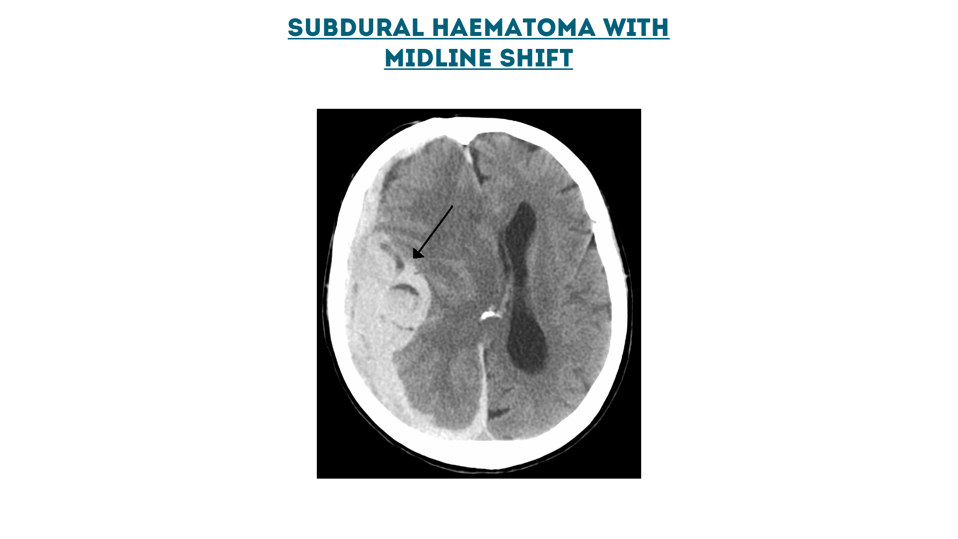
Subdural haematoma

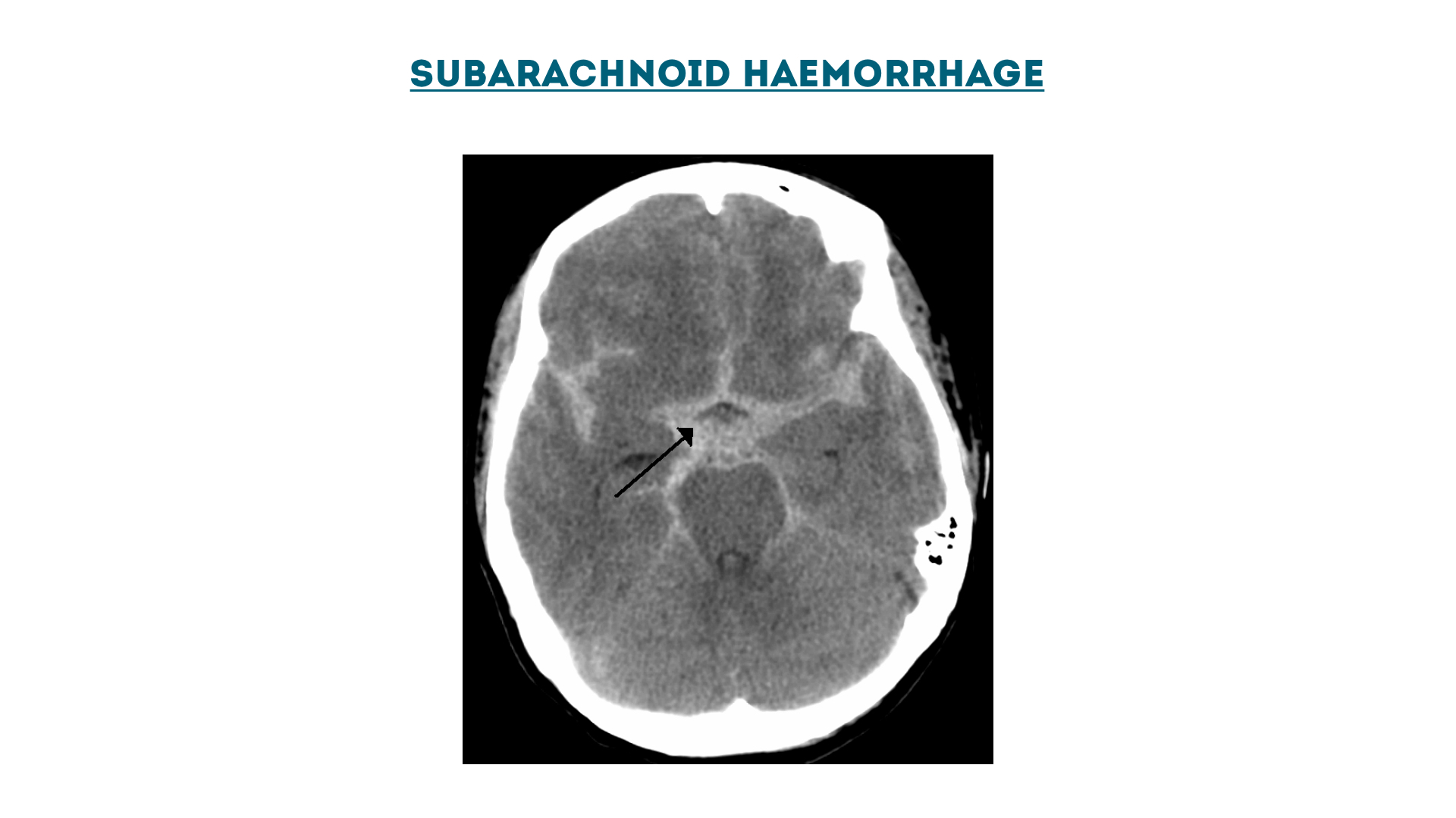
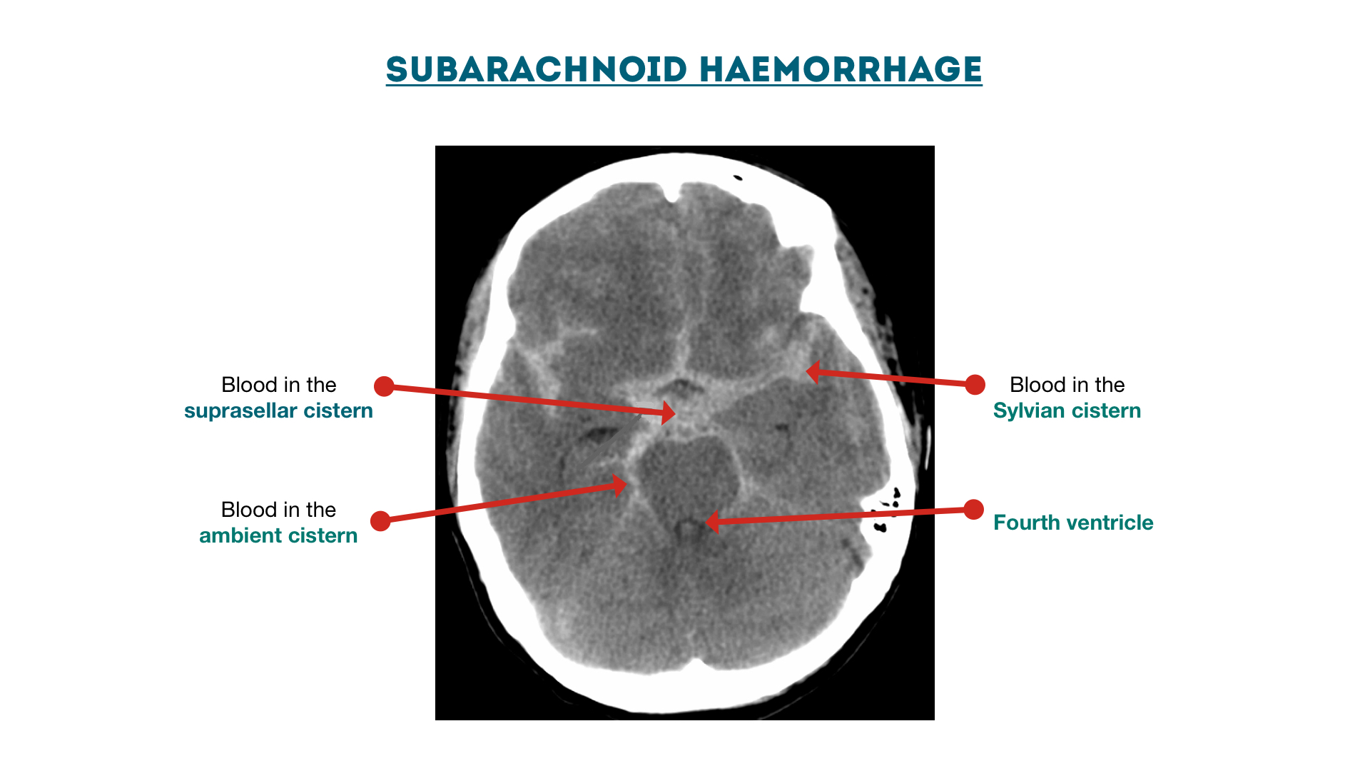
Subarachnoid haemorrhage

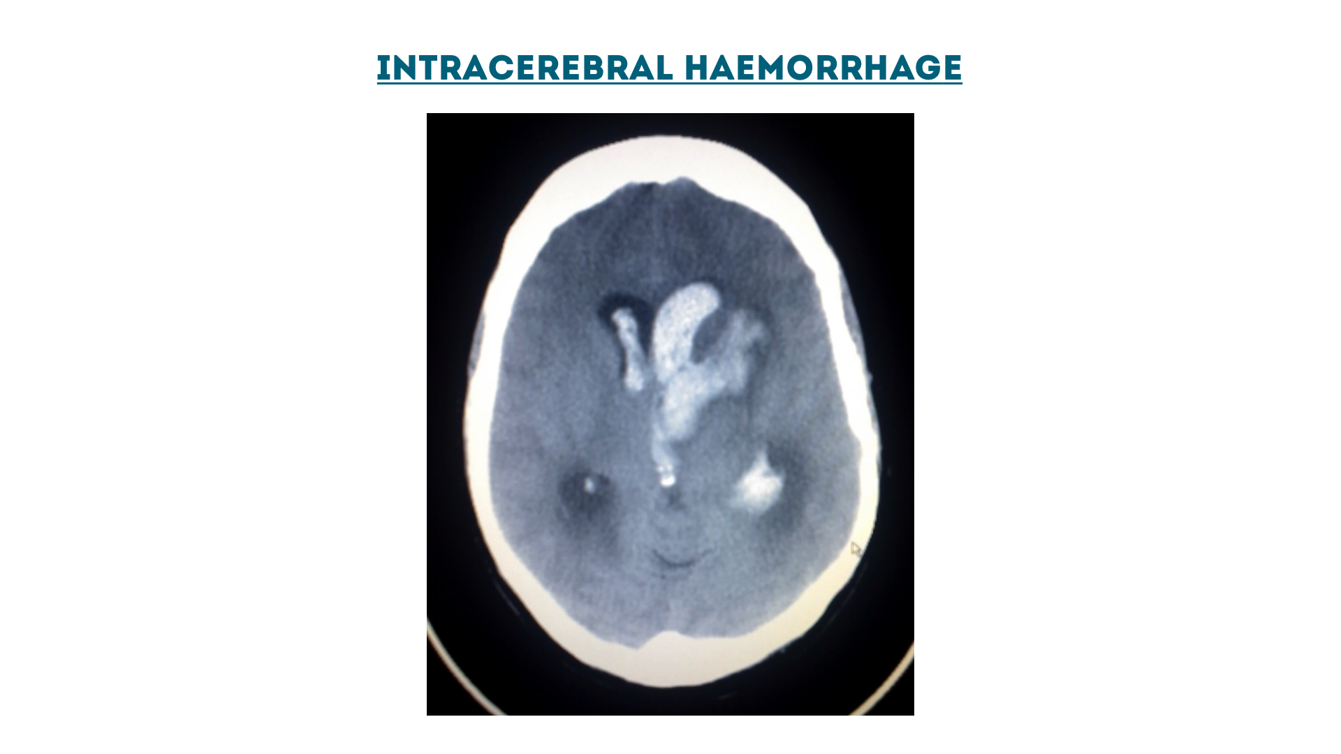
Intracerebral haemorrhage

Cisterns

Brain

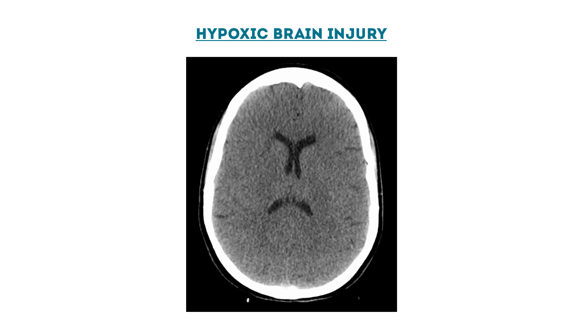
Hypoxic Brain Injury

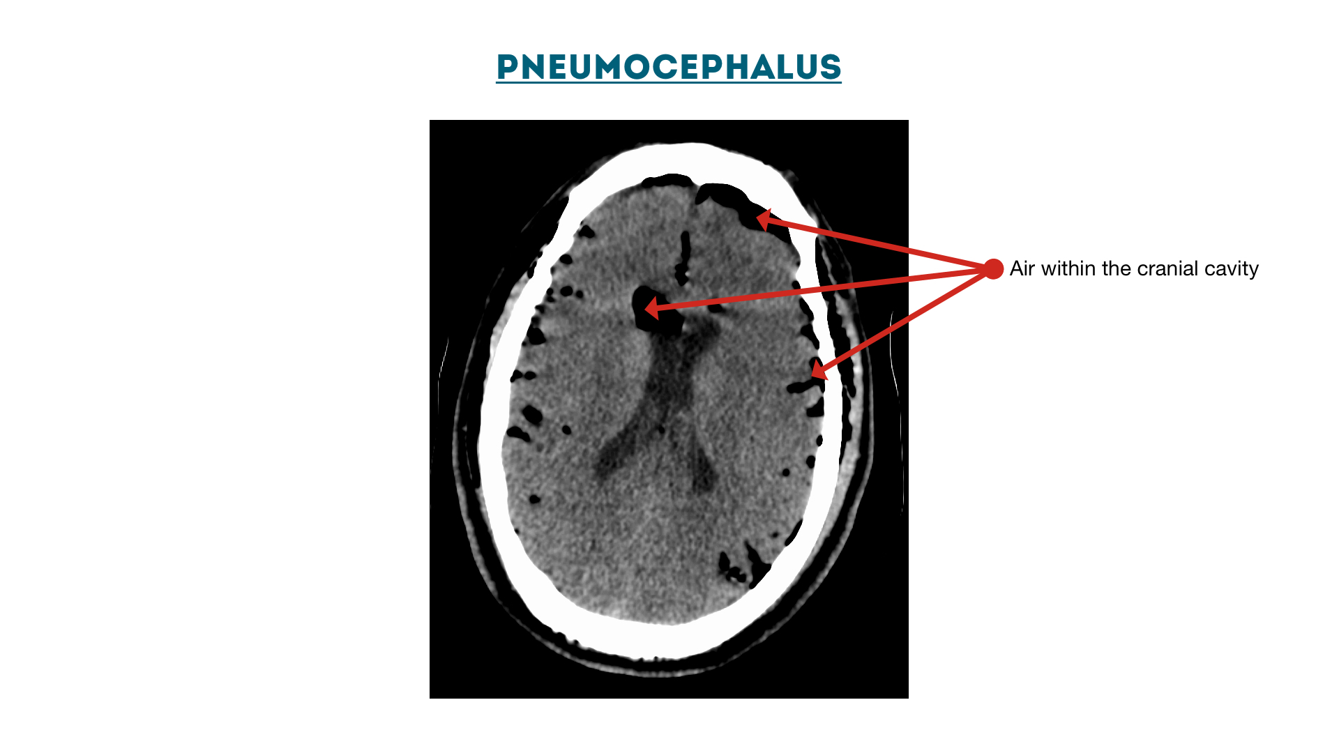
Pneumocephalus

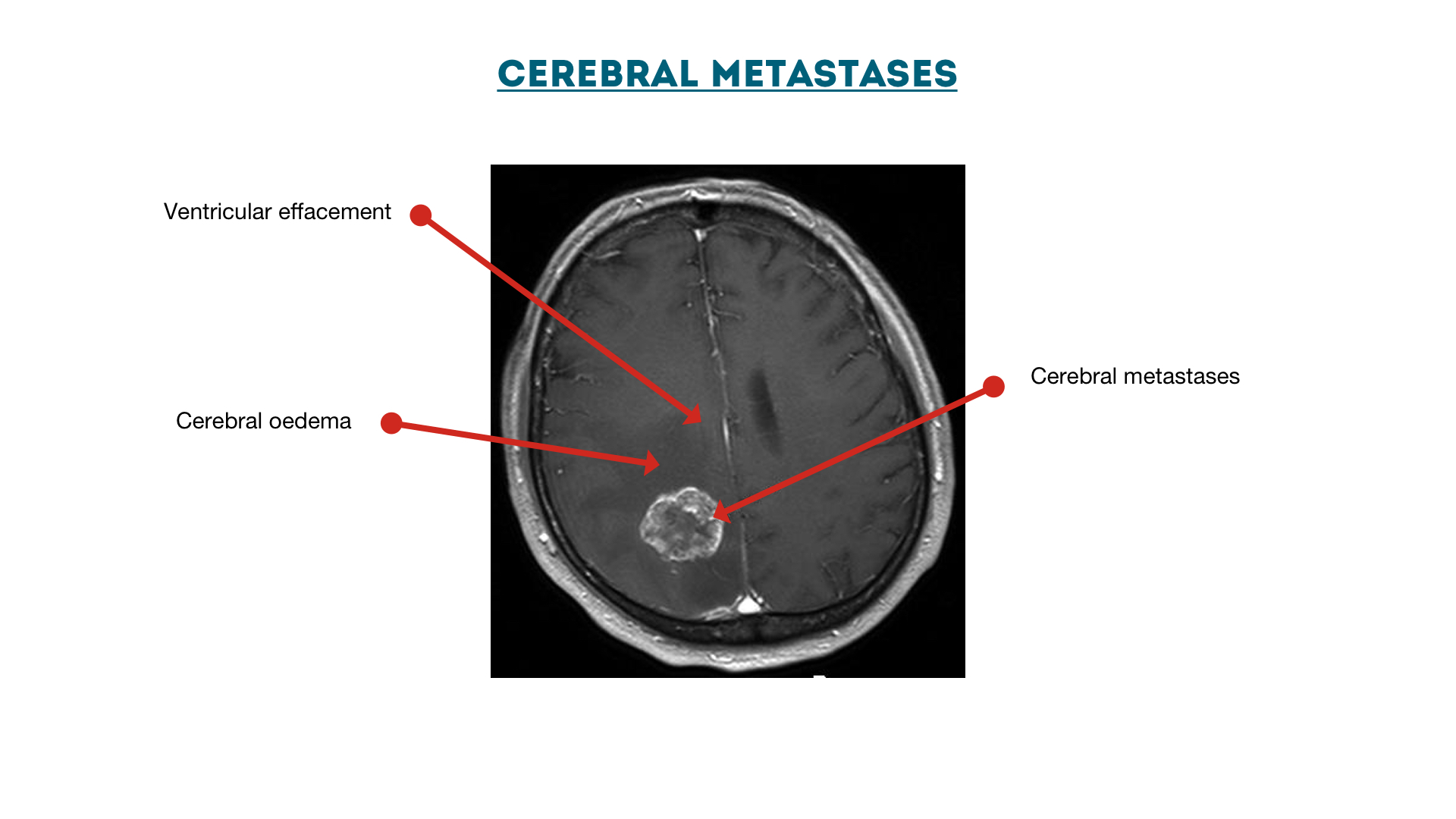
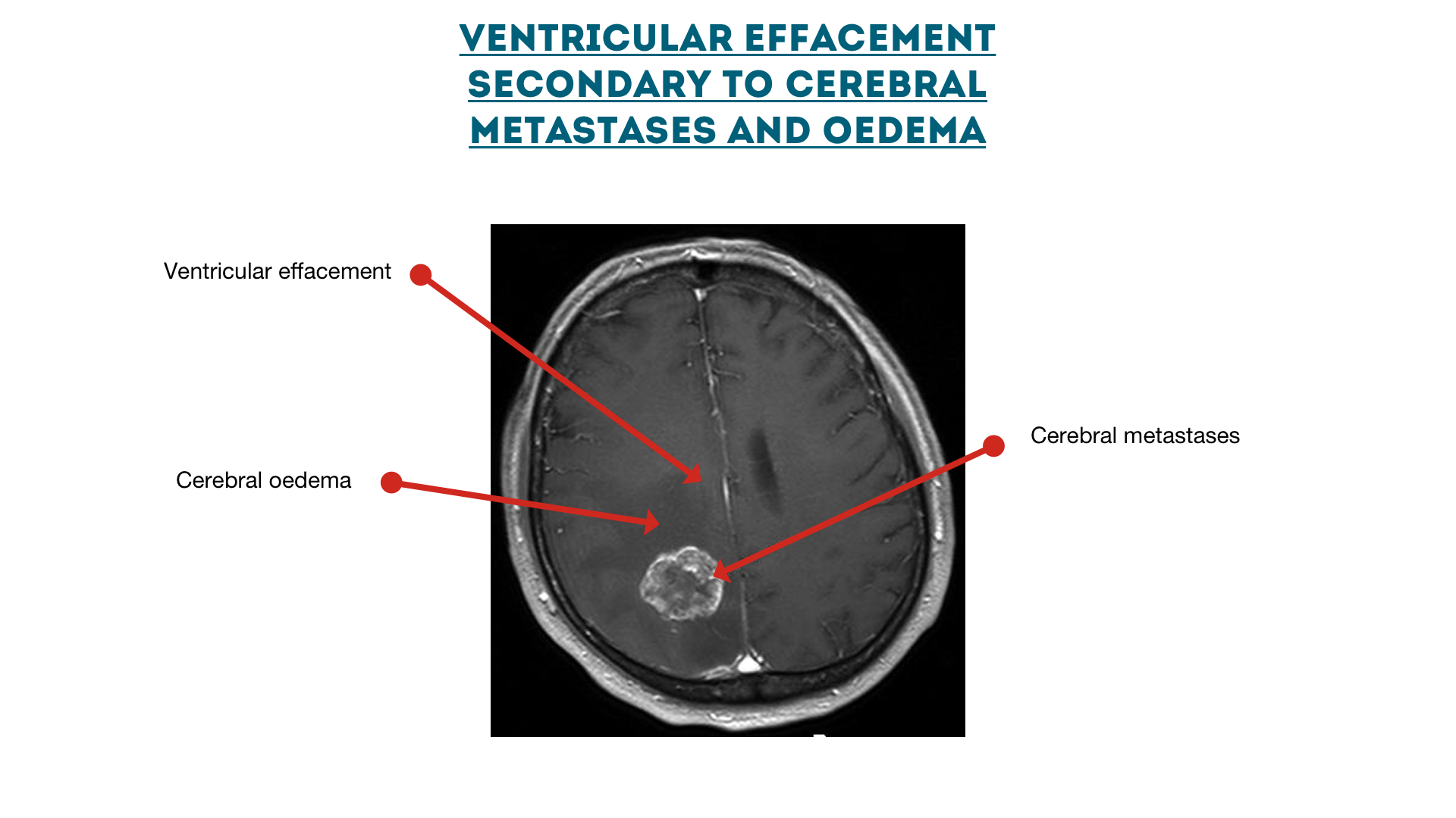
Cerebral metastases with oedema

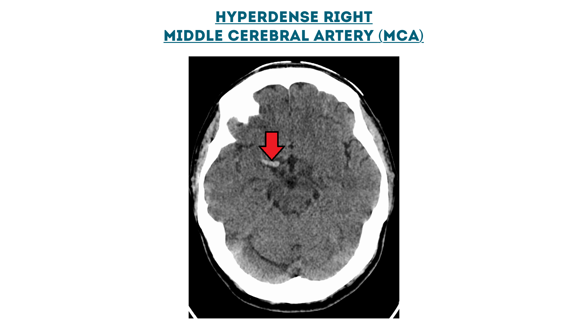
Hyperdense right middle cerebral artery (MCA)

Ventricles

Intracerebral haemorrhage (intraventricular and intraparenchymal)

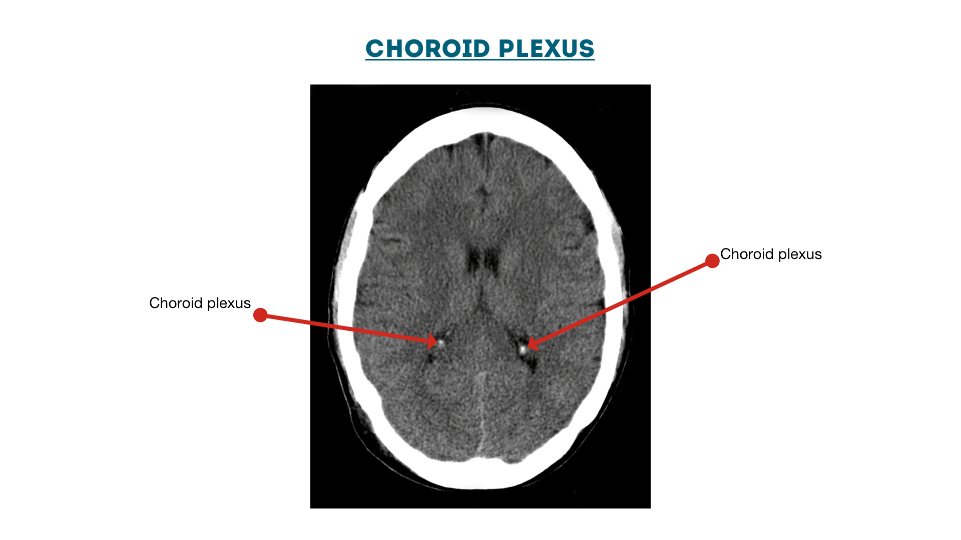
Choroid Plexus

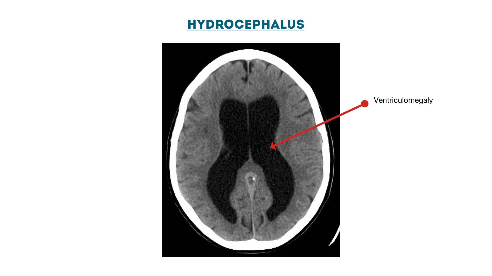
Hydrocephalus: enlarged ventricles (ventriculomegaly)

Ventricular effacement secondary to cerebral metastases

Reference

• https://geekymedics.com/ct-head-interpretation/

2. Intracranial Hemorrhage Detection by 3D Voxel Segmentation on Brain CT Images

Problem Statement

Intracranial hemorrhage (ICH) is a vital disease which occurs due ot leakage or rupture of blood vessels within the brain tissues.

This paper addresses the problem of automatically detecting the hemmorhage regions from brain CT images using image segmentation techniques.

Related Work

Most of the related works use very simple segmentation algorithms such as clustering and thresholding so that these methods may perform well on standard images but cannot deal with complex situations such as the hemorrhage region overlaps with the brain tissues or the edge of hemorrhage is not discriminative enough.

Also, these methods only deal with 2-dimensional images.

Method

1. Use FCM to cluster pixels for the intracranial region.
2. Use Otsu’s adaptive thresholding to further segment the hemorrhagic region.
3. Series of 2D images are reconstructed into 3D spaces by using MITK. Only the detected regions need to be reconstructed which saves big amount of time.
4. For refined segmentation, Simple Linear Iterative Clustering (SLIC) approach is used as part of supervoxel algorithm.
5. Then, to further refine segmentation, graph cuts are used.

Dataset

Experiments are carried out on a Brain CT database, which consists of CT images of 20 patients who were suffering with ICH. For each patient, there are 250 to 350 2D CT images according to different head size of each patient. This database is collected from Department of Neurosurgery, CPLA No. 98 Hospital, Huzhou, China. The CT images are acquired from CT scanners manufactured by General Electric (GE) medical systems. Each CT image is stored in DICOM file format, with a size of 512×512 and spatial resolution of 0.468×0.468mm. Based on the agreements of patients, part of this database is online upon requests.

Metrics Used

1. True Positive Fraction (TPF)
2. False Fraction (FF)
3. Segmentation Error (SE)

3. Deep Learning for Hemorrhagic Lesion Detection and Segmentation on Brain CT Images

Problem Statement

Stroke is a disease caused by the decrease of blood flow to the brain. A stroke occurs when the blood supply to part of the brain is suddenly interrupted (ischemic stroke) or when a blood vessel in the brain bursts and spills blood into the spaces surrounding brain cells (hemorrhage stroke).

This paper proposes a U-Net based deep learning framework to automatically detect and segment hemorrhage strokes in CT brain images.

Related Work

Few works use 3D CNN for segmentation. However, due to the high computational cost and GPU memory consumption, the depth of the 3D network is limited compared to that of a 2D network. This makes the 3D network impractical in stroke diagnosis. Besides, due the high complexity of 3D networks, it is even more difficult to get an adjustable parameter for the ideal model to get the best performance.

There is also less work done on hemorrhage stroke semantic segmentation and no semantic segmentation approach has shown competitive performance compared with human experts.

Method

1. Input : Instead of using the original CT images, this paper concatenates the flipped image with the original CT slice as input of the network, which validate the effective of symmetric structure in contrast enhancement. Aside from data argumentation, data balance was also discussed in the proposed model.
2. Structure of the model: Based on the most state-of-the-art UNet model, various kinds of modified architectures with different layers, batch normalization, dilation rates and pre-train models were compared and evaluated, which provide a solution on how to increase the respective filed and preserves more information of lesion characteristic
3. Training process: To reduce the effect of the normal area in the brain image, the conditional generative adversarial nets (GAN) were modified by using UNet as a generator. Then the discriminator can be used to exploit higher-order inconsistencies in the samples synthesized by the generator. Patch training and the activation layer of LeakyReLu are used in the training process to improve the performance in the small lesion part of the image.

Dataset

1. Dataset1: A single comprehensive stroke center dataset is collected, which includes the brain CT images of 190 patients presenting acute stroke symptoms to the emergency department (58 with hemorrhage, 101 normal). Strokes occur in different locations, with large differences in shape, size, contrast, and unclear boundaries compared with normal parts of the brain across different patients. Interpreting a CT image for hemorrhagic stroke requires thorough evaluation, especially to identify the small area of hemorrhage with low contrast from normal brain tissue. For lesions that do not have distinguished edges or contrast with normal parts, it is very difficult to confirm even by an expert. Based on that, stroke neurologists divided the dataset into two different subsets: one containing subjects with large lesions that are easily diagnosed and one containing subjects with small lesions that are hard to diagnose. The former had 71 images and the latter had 49 images. Manual segmentation of the hemorrhage CT scans was used as the ground truth to evaluate different UNet structures.
2. Dataset2: A benchmark dataset, which includes 36 scans for patients diagnosed with intracranial hemorrhage with the following types: Intraventricular, Intraparenchymal, Subarachnoid, Epidural and Subdural. Each CT scan for each patient includes about 30 slices with 5 mm slice-thickness. The mean and std of patients’ age were 27.8 and 19.5, respectively. 46 of the patients were males and 36 of them were females. Each slice of the non-contrast CT scans was examined by two radiologists who recorded hemorrhage types if hemorrhage occurred or if a fracture occurred.

Metrics Used

1. Location Accuracy (LA)
2. Dice similarity coefficient (DSC)
3. Intersection over Union (IoU)
4. Precision and Recall

4. Autoencoders for unsupervised anomaly segmentation in brain MR images: A comparative study

Problem Statement

Supervised deep learning have few disadvantages like their training calls for large and diverse annotated datasets which are scarce and costly to obtain. Also, the resulting models are limited to the discovery of lesions which are similar to those in the training data.

The underlying idea thereby is to model the distribution of healthy anatomy of the human brain with the help of deep (generative) representation learning. Once trained, anomalies can be detected as outliers from the modeled, normative distribution. AEs and their generative siblings have emerged as a popular framework to achieve this by essentially learning to compress and reconstruct MR data of healthy anatomy. The respective methods can essentially be divided into two categories:

1. Reconstruction-based approaches compute a pixel-wise discrepancy between input samples and their feed-forward reconstructions to determine anomalous lesions directly in image-space
2. Restoration-based methods try to alter an input image by moving along the latent manifold until a normal counterpart to the input sample is found, which in turn is used again to detect lesions from the pixel-wise discrepancy of the input data and its healthy restoration.

Related Work

All of the UAD based methods report promising performances. However, results can hardly be compared and drawing general conclusions on their strengths & weaknesses is barely possible. This is hindered by the following issues:

1. most of the works rely on very different datasets with barely overlapping characteristics for their evaluation
2. are evaluated against different pathologies
3. operate on different resolutions
4. utilize different model architectures with varying model complexity.

The intent of this work is to establish comparability among a broad selection of recent methods by utilizing a single network architecture, a single resolution and the same dataset(s).

Comparisons

1. Modeling healthy anatomy
   1. AE
   2. VAE
   3. AAE
   4. AnoVAEGAN
   5. Context AE
   6. GAN
2. Anomaly segmentation
   1. Reconstruction Based Methods
      1. Monte Carlo Methods
         1. Bayesian AE
         2. Bayesian VAE
      2. Gradient Based Methods
   2. Restoration Based Methods

Datasets

1. Healthy, MS & GB : The primary dataset used in this comparative study is a homogenous set of MR scans of both healthy and diseased subjects, produced with a single Philips Achieva 3T MR scanner. It comprises FLAIR, T2- and T1-weighted MR scans of 138 healthy subjects, 48 subjects with MS lesions and 26 subjects with Glioma. All scans have been carefully reviewed and annotated by expert Neuro-Radiologists. Informed consent was waived by the local IRB.
2. MSLUB : The second MRI dataset consists of co-registered T1, T2 and FLAIR scans of 30 different subjects with MS. Images have been acquired with a 3T Siemens Magnetom Trio MR system at the University Medical Center Ljubljana (UMCL). A gold standard segmentation was obtained from consensus segmentations of three expert raters.
3. MSSEG2015 : The third MRI dataset in our experiments is the publicly available training set of the 2015 Longitudinal MS lesion segmentation challenge, which contains 21 scan sessions from 5 different subjects with T1, T2, PD and FLAIR images each. All data has been acquired with a 3.0 Tesla Philips MRI scanner.

Metrics

1. Precision-Recall-Curves (PRC)
2. AUPRC
3. DICE-score
4. Receiver-Operating-Characteristics (ROC)
5. AUROC
6. L1-reconstruction

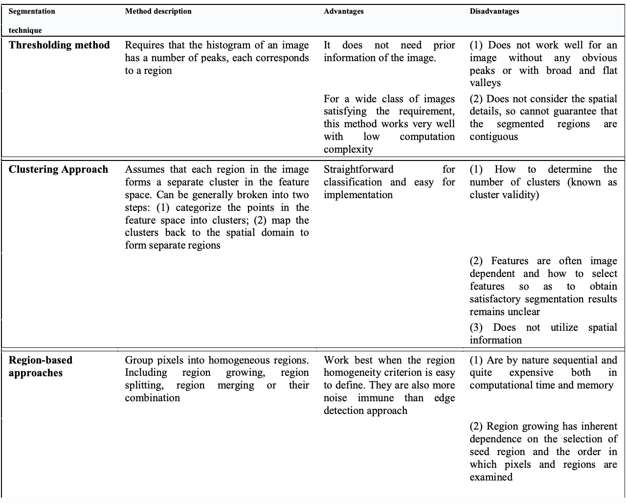
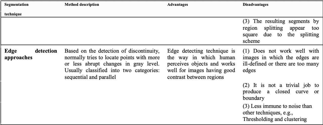
5. Medical Image Segmentation: A Review

The main components of the paper are listed in the table :

6. Intensity population based unsupervised hemorrhage segmentation from brain CT images

Problem Statement

This paper suggests a lightweight and a sufficiently accurate method for detection of hemorrhage.

Related Work

Hemorrhage finding is mostly done by locating threshold on the histogram. This is done automatically through machines artificial intelligence using different algorithms like fuzzy C-means, Hopfield neural network, maximum entropy, fuzzy maximal likelihood estimation, probabilistic neural network, genetic algorithm.

To detect hemorrhage few more approaches to knowledge based detection, histogram-based K-means clustering, wavelet-based texture analysis are also proposed in different works.

Unsupervised clustering and backtracking tree search method are also reported in some papers.

Deep learning methods are also in used for segmentation. Most of them are supervised techniques which require a large number of data. This requirement itself is a disadvantage of these methods. Different deep learning techniques are outperformed by the traditional k-means method used in an unsupervised system which involves a limited number of data.

Method

1. HU based windowing is done.
2. Skull stripping is followed using slopes and thresholds.
3. Then brain segmentation is done by finding the largest connected component.
4. Background removing is then done using threshold from intensity population.
5. Further hemorrhage is segmented using population histogram. This method uses deviation between actual and expected Population.
6. In order to further refine results, localtion finalization is also done on the dataset level.

Dataset

Datasets of multi-slice brain CT images are taken for hemorrhage detection. Images are scanned by a 64 slice CT scanner with slice thickness 5 mm. The original DICOM (Digital Imaging & Communication in Medicine) images, provided by radiology department of Postgraduate Institute of Medical Education and Research (PGIMER), Chandigarh, India

Metrics

1. Sensitivity
2. Specificity
3. Dice coefficient
4. Accuracy

7. Multi-view fusion segmentation for brain glioma on CT images

Problem Statement

2D CNN-based methods address image sequences by segmenting the different slice images separately. In contrast, 3D CNN-based methods segment the entire image sequence as a whole. Because of the resulting drop in spatial information, 2D CNN-based methods generally have lower performance than 3D-based methods. However, 3D-based methods require a more complex network structure and are more challenging to train.

To address the above problems, the paper proposes an encoder decoder brain tumor segmentation framework with multiview fusion.

Related Work

There are a lot of traditional ways of doing segmentation. Although traditional methods have made great achievements in segmenting brain tumors, there remain several drawbacks. The segmentation performances of the above methods rely heavily on hand-crafted features, meaning that weak features may cause failures in subsequent processes. Furthermore, the manual selection of features is time-consuming and subjective, which means that it is difficult to improve the performance of these approaches.

Hence, paper propose multi-view fusion using deep neural networks.

Method

1. Data is preprocessed using windowing and other basic steps.
2. Encoder-decoder framework is used where the input is the multi-view image including the previous, current and following image is used.
3. More details are clearly mentioned in the paper (Supervised technique).

Dataset

The data used in the experiments came from a total of 225 patients with pathologically proven glioma cancer who were treated with postoperative radiotherapy from February 2016 to April 2019 at the Department of Radiation Oncology of West China Hospital, Sichuan University.

Metrics used

1. Dice similarity coefficient (DSC)
2. True positive volume fraction (TPVF)
3. Positive predictive value (PPV)

8. Accelerating Prediction of Malignant Cerebral Edema After Ischemic Stroke with Automated Image Analysis and Explainable Neural Networks

Problem Statement

Cerebral edema develops in the hours to days after acute ischemic stroke and may result in midline shift and cerebral herniation. Te volume of cerebrospinal fuid (CSF) relative to total cranial volume, termed intracranial reserve, is emerging as a useful biomarker, with lower reserve on baseline imaging increasing the risk for subsequent edema-related decompensation.

Paper proposes a pilot study evaluating the impact of two significant innovations to the imaging-based prediction algorithm: the first is to incorporate the hemispheric CSF ratio (i.e., the ratio of CSF volumes between the two hemispheres), not just total CSF displacement; the second is to employ neural networks that can integrate serial clinical and imaging features in complex, dynamic, and nonlinear ways to enhance prediction beyond what is capable by traditional regression models.

Method

1. Imaging analysis is done first and CSF ratio is calculated by hemisphere.
2. Fully-connected neural network and LSTMs were used for prediction.

Dataset

Patients enrolled in an international prospective inpatient stroke cohort (the Genetics of Neurological Instability after Ischemic Stroke [GENISIS]) study between 2008 and 2017 were retrospectively evaluated for eligibility. All participants presented within 6 h of stroke onset. They selected those with baseline CT within 12 h of onset and follow-up CT within 48 h from three sites. At two sites, it was standard protocol to obtain repeat CT at 24 h after thrombolytic and/or endovascular therapies. At the third, it was performed at the stroke physician’s discretion and for any deterioration or concerns for neurological complications. They excluded participants if onset time was unknown, if the baseline CT scan already showed well-developed infarction (suggesting that the time of stroke onset was likely earlier than annotated; other acute stroke-related hypodensity was acceptable), if the stroke was located in the brainstem or cerebellum, or if the final discharge diagnosis was not stroke. NIHSS scores were obtained at baseline (within 6 h of stroke onset or last time known to be well) and at 24 h. Serum glucose and blood pressure were obtained on presentation. All participants provided informed consent. Tey were observed prospectively for neurological deterioration or death during hospital admission. Surgery (DHC) was considered in cases of clinical deterioration with midline shift and not preemptively prior to deterioration. Our primary end point was the development of malignant edema leading to either DHC and/or death in the presence of midline shift of 5 mm or greater. This retrospective imaging sub-study was approved by the coordinating site’s institutional review board.

Metrics

1. Recall
2. Precision
3. Specificity
4. Accuracy
5. AUROC
6. AUPRC
7. Brier Score

9. Automated medical image segmentation techniques

The paper talks about MRI and CT medical images.

MR acquisition takes considerably longer time as compared to CT and in case of MR it is more difficult to obtain uniform image quality. CT scans are particularly used in imaging and the diagnosis of following body parts: brain, liver, chest, abdomen and pelvis, spine and also for CT based angiography.

In case of brain imaging, CT scans are typically used to detect: bleeding, brain damage and skull fracture in patients with head injuries; bleeding caused by a ruptured or leaking aneurysm in a patient with a sudden severe headache, blood clot or bleeding within the brain shortly after a patient exhibits symptoms of a stroke, brain tumors, cyst, diseases related to malformations of the skull, enlarged brain cavities (ventricles).

CT scanning is fast and simple, provides more detailed information on head injuries, and stroke; can reveal internal injuries and bleeding quick enough to help save lives in emergency cases.

Segmentation Techniques

1. Methods based on gray Level features
   1. Amplitude segmentation based on histogram features
   2. Edge based segmentation
      1. Edge relaxation
      2. Border detection method
      3. Hough transform based
   3. Region based segmentation
      1. Region merging
      2. Region splitting
      3. Split and merge
2. Methods based on texture features
   1. Statistical approach
   2. Syntactic or structural approach
   3. Spectral approach
3. Model based segmentation
4. Atlas based segmentation
5. Artificial Intelligence Tools for Segmentation and Classification
   1. Supervised methods
   2. Unsupervised methods

10. Application of Machine Learning to Automated Analysis of Cerebral Edema in Large Cohorts of Ischemic Stroke Patients

The paper presents results of their preliminary processing pipeline that was able to efficiently extract CSF volumetrics from an initial cohort of 155 subjects enrolled in a prospective longitudinal stroke study.

The paper demonstrated that the volume of CSF displaced up to the time of maximal edema closely correlated with extent of midline shift.

The image processing pipeline to analyze CSF volumes :

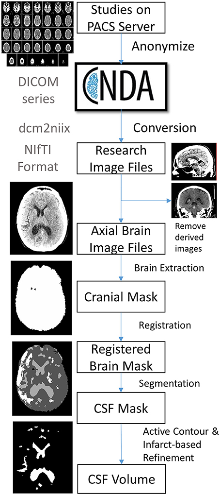
The steps outlined are :

1. Subjects and Data collection
2. DICOM conversion
   1. using dcm2niix software
3. Image Selection
4. Brain extraction and Perimeter Registration
   1. Skull stripping - k means clustering
   2. Registration - using Advanced Normalized Toolkit (ANTS)
5. CSF segmentation
   1. Use random forest machine learning - Cited in the paper.
   2. Results refined using an active contour method and cleaned using a manually drawn mask of the infract hypodensity.
6. Volumetric Analyses
   1. The number of pixels in each compartment (intracranial compartment, CSF, infarct) is extracted from each image mask. This is then converted into volume using the pixel dimensions in the image header.

11. Quantitative Serial CT Imaging-Derived Features Improve Prediction of Malignant Cerebral Edema after Ischemic Stroke

The paper aims to develop a multivariable machine learning model for predicting malignant cerebral edema using a combination of clinical and quantitative imaging variables extracted from CTs at baseline and 24-h.

The pipeline for imaging analysis is given in the paper. This included first extraction of the intracranial supratentorial space using k-means clustering for skull removal followed by registration of each baseline image to atlas templates for removal of infratentorial and noncranial structures. Te follow-up images were then coregistered to the baseline for each participant to ensure similar brain volumes were analyzed. These cranial regions then underwent automated segmentation into CSF and brain compartments. If more than one scan was performed at a time point (e.g., normal axial brain and thin slices), they selected scans with 3–5-mm slice thickness, for consistency. The intracranial reserve was calculated as the proportion of cranial volume comprised by CSF. Percent change in CSF volume from baseline to 24-h was calculated as ∆CSF. Midline shift was measured manually by a single trained investigator at the level of the septum pellucidum. Infarct-related hypodensity was manually outlined slice-by-slice to provide lesion volume (a combination of infarct and edema).

Te dataset was complete except for a few missing data points: for NIHSS and glucose. Values were imputed for each missing feature using the three closest data points, using the K-Nearest Neighbor (KNN) algorithm. All features were then standardized to improve stability of model training. Te dataset was partitioned into ten folds, and tenfold cross-validation was employed to train and internally validate each model.

They applied logistic regression to provide probabilistic binary outputs using a one-layer neural network with softmax activation, implemented within the Keras machine-learning platform.

AUPRC is used as a metric.

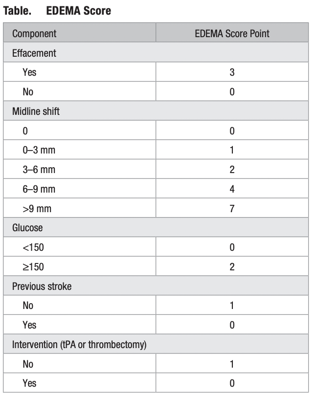
12. Enhanced Detection of Edema in Malignant Anterior Circulation Stroke (EDEMA) Score A Risk Prediction Tool

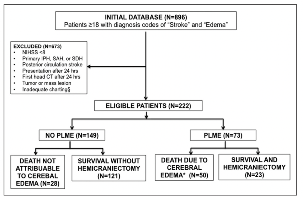
The purpose of this study was to develop a practical risk prediction tool that can aid in rapidly and accurately triaging patients at high risk for potentially lethal malignant edema (PLME) within the first 24 hours of stroke with high positive predictive value.

Eligibility Criteria :

EDEMA Score :